|
Artificial dataset A
|
Artificial dataset
B
|
ICA VS. PCA COMPARISON
In this webpage you can find some experimental results that show how ICA and PCA behave on different classification tasks relative to appearance-based recognition systems.
1. DATASETS USED FOR THE EXPERIMENTS
2. ALGORITHMS USED FOR THE EXPERIMENTS
1. DATASETS USED FOR THE EXPERIMENTS
|
Artificial dataset A
|
Artificial dataset
B
|
|
Real data of object images (COIL-100)
|
|
Real data of face images (ORL faces)
|
2. ALGORITHMS USED FOR THE EXPERIMENTS
Two ICA implementations have been used for the experiments:
The matlab source code used for the experiments is available through the links provided in this pages.
This code has been tested using Matlab 6.5 running under WindowsXP.
You may use other ICA implementations just by modifying the code and adding your ICA functions.
Two different global experiments have been performed:
ICA vs. PCA comparison without feature selection (in sections 5.1 and 5.2)
In these first experiments, both ICA and whitened PCA are used to compress the data, and all the components are used for classifying the examples. The classifier used is a 1-NN with Euclidean distance. The results shown in next sections are clear: when a rotational invariant classifier is used (as 1-NN with L2-norm) the classification results of FastICA/whitened PCA are equivalent, while the difference between Infomax and whitened data es significant but small.
ICA vs. PCA comparison with feature selection (in sections 5.3 and 5.4)
In this second set of experiments, both ICA and whitened PCA are used to compress the data but not all the components are used for classification. The goal is to detect possible advantages of ICA over whitened PCA when only a subset of the components are used for classification. In other words, the goal is to check whether ICA is able to extract certain components that are particularly appropriate for separating the different classes in the dataset. The results of the experiments performed show that ICA does not necessarily outperforms whitened PCA. This fact is clearly shown when using the artificial datasets.
The matlab code used for the experiments is available here:
It is very easy to use. The main function is "example.m", which only accepts three parameters:
Apart from these parameters, different options of the experiment (number of classes, number of vectors, etc) can be adjusted just by modifying the "example.m" function, which is fully commented.
The results are shown in different plots. The number of plots may vary depending of the experiment carried out.
We can run the experiment without modifying the parameters just by typing:
>> example(1,1,0)
This command runs the experiment for the first dataset (Artificial dataset A) using FastICA, without feature selection.
The output should be the following, where the classification results are highlighted in yellow:
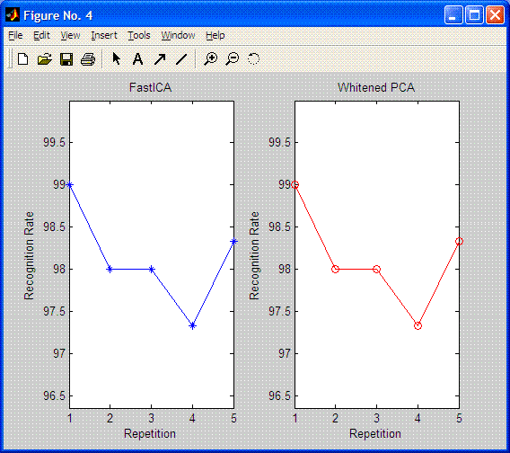
| Artificial dataset A Doing PCA and ICA.... Warning: You are not working with images. I will compute PCA in the regular way. Number of signals: 2 Number of samples: 600 Calculating covariance... Dimension not reduced. Selected [ 2 ] dimensions. Smallest remaining (non-zero) eigenvalue [ 0.481352 ] Largest remaining (non-zero) eigenvalue [ 1.7142 ] Sum of removed eigenvalues [ 0 ] [ 100 ] % of (non-zero) eigenvalues retained. Whitening... Check: covariance differs from identity by [ 8.88178e-016 ]. Number of signals: 2 Number of samples: 600 Calculating covariance... Dimension not reduced. Selected [ 2 ] dimensions. Smallest remaining (non-zero) eigenvalue [ 1 ] Largest remaining (non-zero) eigenvalue [ 1 ] Sum of removed eigenvalues [ 0 ] [ 100 ] % of (non-zero) eigenvalues retained. Whitening... Check: covariance differs from identity by [ 9.99201e-016 ]. Used approach [ defl ]. Used nonlinearity [ pow3 ]. Starting ICA calculation... IC 1 .....computed ( 5 steps ) IC 2 ..computed ( 2 steps ) Done. Adding the mean back to the data. Feature extraction is finished. Classifying...... REPETITION no. 1 FastICA Recognition rate:99.00 Whitening Recognition rate :99.00 REPETITION no. 2 FastICA Recognition rate:98.00 Whitening Recognition rate :98.00 REPETITION no. 3 FastICA Recognition rate:98.00 Whitening Recognition rate :98.00 REPETITION no. 4 FastICA Recognition rate:97.33 Whitening Recognition rate :97.33 REPETITION no. 5 FastICA Recognition rate:98.33 Whitening Recognition rate :98.33 For all the repetitions: FastICA Recognition rate:98.13 ± 0.27 Whitening Recognition rate :98.13 ± 0.27 |
Apart from this command line information, some figures are displayed:


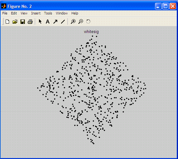
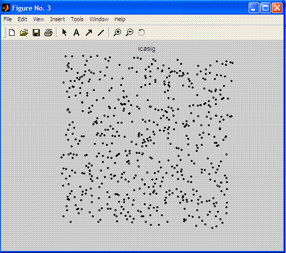
The first two plots are shown just when the number of components used in the transformation is 2 (n_vectors=2;).
The last plot gives us the recognition rate of each experiment or repetition (5 in this case, nr=5). Feature extraction process is performed just once, using all the available examples in each class. Then, different repetitions run the classifier with randomly selected train and test sets. In this example 50% of the data is use to train the 1-NN and the other 50% is used to test (per_test=0.5;).
Both this figure and the command line information show clearly that ICA and PCA (WHITENING) perform equally for FastICA algoritm.
In the following sections there are some experimental results obtained by means of our code and using the above datasets:
5.1.Artificial datasets without feature selection
5.2 Real data without feature selection
5.3.Artificial datasets using feature selection
5.4 Real data using feature selection
Last updated, - April,28 -2006